Your first XPD pattern

In this small example, you will learn how to produce a polar scan, ie you will plot the number of photo-electrons as a function of the \(\theta\) angle. We will do this calculation for a bulk copper (001) surface.

This is a small script of roughly 15 lines (without comments) just to show you how to start with the msspec package. For this purpose we will detail all steps of this first hands on as much as possible.

Start your favorite text editor to write this Python script.

Begin by typing:

# coding: utf8

from msspec.calculator import MSSPEC
from msspec.utils import *

Every line starting by a ‘#’ sign is considered as a comment in Python and thus is ignored… except the first line with the word ‘coding’ right after the ‘#’ symbol. It allows you to specify the encoding of your text file. It is not mandatory but highly recommended. You will most likeley use an utf-8 encoding as in this example.

For an MsSpec calculation using ASE, msspec modules must be imported first. Thus, line 3 you import the MSSPEC calculator from the calculator module of the msspec package. MSSPEC is a class.

We will also need some extra stuff that we load from the utils module (line 4).

We need to create a bulk crystal of copper atoms. We call this a cluster. This is the job of the ase module, so load the module

from ase.build import bulk
from ase.visualize import view

a0 = 3.6 # The lattice parameter in angstroms

# Create the copper cubic cell
copper = bulk('Cu', a=a0, cubic=True)
view(copper)

In line 6 we load the bulk() function to create our atomic object and, in line 7, we load the view() function to actually view our cluster.

The creation of the cluster starts on line 12. We create first the copper cubic cell with the The bulk() function. It needs one argument which are the chemical species (‘Cu’ in our example). We also pass 2 keyword (optional) arguments here:

• The lattice parameter a in units of angströms.

• The cubic keyword, to obtain a cubic cell rather than the fully reduced one which is not cubic

From now on, you can save your script as ‘Cu.py’ and open a terminal window in the same directory as this file. Launch your script using ‘python’ or ‘msspec -p’ (depending on your installation):

python Cu.py

or

msspec -p Cu.py

and a graphical window (the ase-gui) should open with a cubic cell of copper like this one:

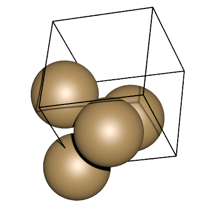
Figure 1.

Obviously, multiple scattering calculations need more atoms to be accurate. Due to the forward focusing effect in photo-electron diffraction, the best suited geometry for the cluster is hemispherical. Obtaining such a cluster is a straightforward process thanks to the utils.hemispherical_cluster() function. This function will basically create a cluster based on a pattern (the cubic copper cell here).

Modify your script like this and run it again.

# coding: utf8

from msspec.calculator import MSSPEC
from msspec.utils import hemispherical_cluster, get_atom_index

from ase.build  import bulk
from ase.visualize import view

a0 = 3.6 # The lattice parameter in angstroms

# Create the copper cubic cell
copper = bulk('Cu', a=a0, cubic=True)
cluster = hemispherical_cluster(copper, planes=3, emitter_plane=2)

Don’t forget to add the line to view the cluster at the end of the script and run the script again. The hemispherical_cluster() works in 3 simple steps:

1. Repeat the given pattern in all 3 directions

2. Center this new set of atoms and cut a sphere from the center

3. Remove the upper half of the created ‘sphere’.

To get more information about how to use this function, have a look at the The hemispherical_cluster function section in the FAQ.

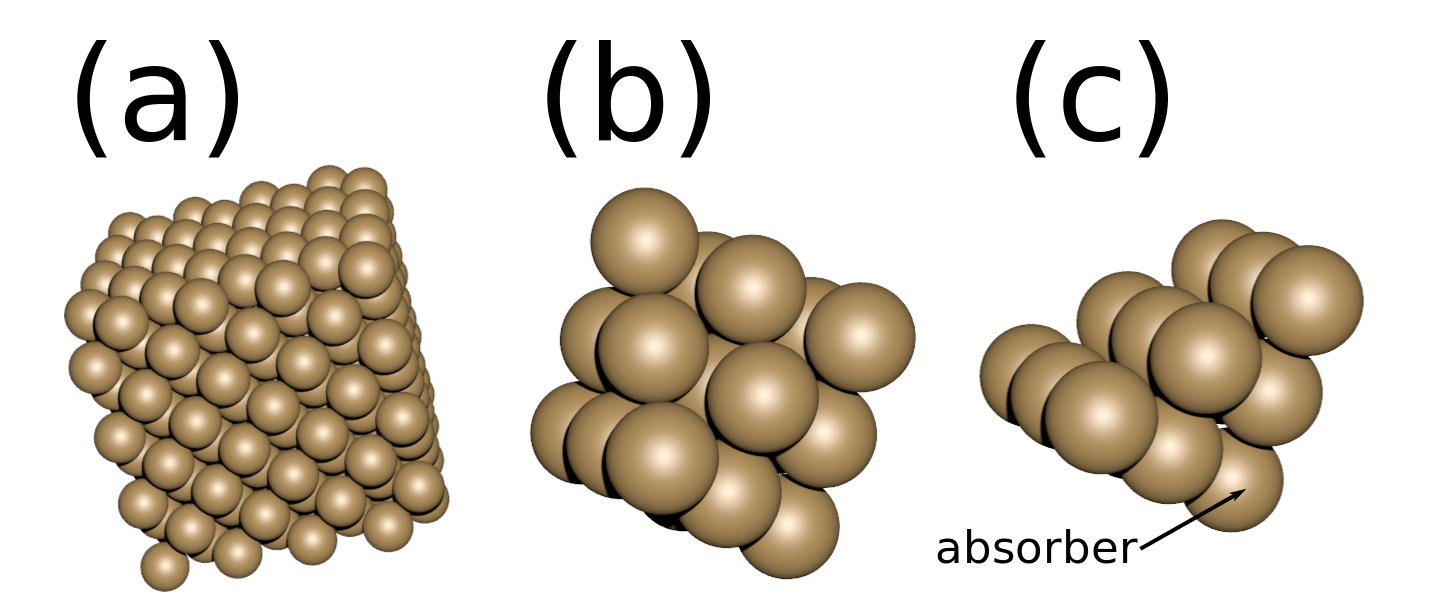
Figure 2. The different steps to output a cluster. a) After repeat, b) after cutting a sphere, c) final cluster

Once your cluster is built the next step is to define which atom in the cluster will absorb the light. This atom is called the absorber (or the emitter since it emits the photoelectron).

To specify which atom is the absorber, you need to understand that the cluster object is like a list of atoms. Each member of this list is an atom with its own position. You need to locate the index of the atom in the list that you want it to be the absorber. Then, put that number in the cluster.absorber attribute

For example, suppose that you want the first atom of the list to be the absorber. You would write:

cluster.absorber = 0

To find what is the index of the atom you’d like to be the absorber, you can either get it while you are visualizing the structure within the ase-gui program (select an atom with the left mouse button and look at its index in the status line). Or, you can use utils.get_atom_index() function. This function takes 4 arguments: the cluster to look the index for, and the x, y and z coordinates. It will return the index of the closest atom to these coordinates. In our example, as we used the utils.hemispherical_cluster() function to create our cluster, the emitter (absorber) is always located at the origin, so defining it is straightforward:

# Set the absorber (the deepest atom centered in the xy-plane)
cluster.absorber = get_atom_index(cluster, 0, 0, 0)

That’s all for the cluster part. We now need to create a calculator for that object. This is a 2 lines procedure:

# Create a calculator for the PhotoElectron Diffration
calc = MSSPEC(spectroscopy='PED')

# Set the cluster to use for the calculation
calc.set_atoms(cluster)

When creating a new calculator, you must choose the kind of spectroscopy you will work with. In this example we choose ‘PED’ for PhotoElectron Diffraction. Other types of spectroscopies are:

• ‘AED’ for Auger Electron Spectroscopy

• ‘APECS’ for Auger PhotoElectron Coincidence Spectroscopy

• ‘EXAFS’ for Extended X-Ray Absorption Fine Structure

• ‘LEED’ for Low Energy Electron Diffraction

Now that everything is ready you can actually perform a calculation. The lines below will produce a polar scan of the Cu(2p3/2) level with default parameters, store the results in the data object and display it in a graphical window.

# Run the calculation
data = calc.get_theta_scan(level='2p3/2')

# Show the results
data.view()

running this script will produce the following output

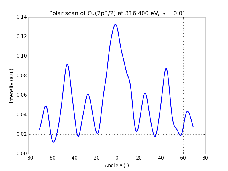
Figure 3. Polar scan of copper (2p3/2)

You can clearly see the modulations of the signal and the peak at \(\theta = 0°\) and \(\theta = 45°\), which are dense directions of the crystal.

By default, the program computes for \(\theta\) angles in the -70°..+70° range. This can be changed by using the angles keyword.

#For a polar scan between 0° and 60° with 100 points
import numpy as np
data = calc.get_theta_scan(level = '2p3/2', theta = np.linspace(0,60,100))

# For only 0° and 45°
data = calc.get_theta_scan(level = '2p3/2', theta = [0, 45])

You probably also noticed that we did not specify any kinetic energy for our photoelectron in this example. By default, the programm tries to find the binding energy (\(E_b\)) of the choosen level in a database and assume a kinetic energy (\(E_k\)) of

\[E_k = \hbar\omega - E_b - \Phi_{WF}\]

where \(\hbar\omega\) is the photon energy, an \(\Phi_{WF}\) is the work function of the sample, arbitrary set to 4.5 eV.

Of course, you can choose any kinetic energy you’d like:

# To set the kinetic energy...
data = calc.get_theta_scan(level = '2p3/2', kinetic_energy = 300)

Below is the full code of this example. You can download it here

# coding: utf8

from msspec.calculator import MSSPEC
from msspec.utils import hemispherical_cluster, get_atom_index

from ase.build  import bulk
from ase.visualize import view

a0 = 3.6 # The lattice parameter in angstroms

# Create the copper cubic cell
copper = bulk('Cu', a=a0, cubic=True)
cluster = hemispherical_cluster(copper, planes=3, emitter_plane=2)

# Set the absorber (the deepest atom centered in the xy-plane)
cluster.absorber = get_atom_index(cluster, 0, 0, 0)

# Create a calculator for the PhotoElectron Diffration
calc = MSSPEC(spectroscopy='PED')

# Set the cluster to use for the calculation
calc.set_atoms(cluster)

# Run the calculation
data = calc.get_theta_scan(level='2p3/2')

# Show the results
data.view()

# Clean temporary files
calc.shutdown()

See also

Atomic Simulation Environnment

Documentation of the ASE module to create your clusters much more.

X-Ray data booklet

Electron binding energies are taken from here.