Playing with the scattering factor

In this tutorial we will play with an important parameter of any multiple scattering calculation: the scattering factor. When a electron wave is scattered by an atom, the electron trajectory is modified after this event. The particle will most likely continue its trajectory in the same direction (forward scattering), but, to a lesser extent and depending on the atom and on the electron energy, the direction of the scattered electron can change. The electron can even be backscattered. The angular distribution of the electron direction after the scattering event is the scattering factor.

In a paper published in 1998, T. Gerber et al. used the quite high backscattering factor of Rhodium atoms to probe the distance of Oxygen atoms adsorbed on a Rhodium surface. Some electrons coming from Oxygen atoms are ejected toward the Rhodium surface. They are then backscattered and interfere with the direct signal comming from Oxygen atoms (see the figure below). They demonstrated both experimentally and numerically with a sinle scattering computation that this lead to a very accurate probe of adsorbed species that can be sensitive to bond length changes of the order of \(\pm 0.02 \mathring{A}\).

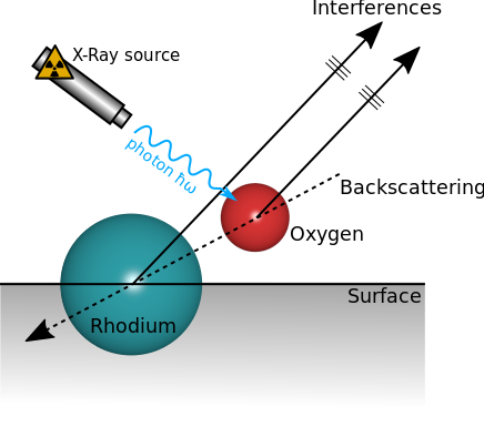
Interferences produced by the backscattering effect.

First, compute the scattering factor of both chemical species, Rh and O.

# coding: utf8

from msspec.calculator import MSSPEC
from ase import Atoms

# Create an atomic chain O-Rh
cluster = Atoms(['O', 'Rh'], positions = [(0,0,0), (0,0,4.)])

# Create the calculator
calc = MSSPEC(spectroscopy = 'PED')
calc.set_atoms(cluster)
cluster.absorber = 0

# compute
data = calc.get_scattering_factors(level='1s', kinetic_energy=723)

data.view()

Running the above script should produce this polar plot. You can see that for Rhodium, the backscattering coefficient is still significant even at quite high kinetic energy (here 723 eV).

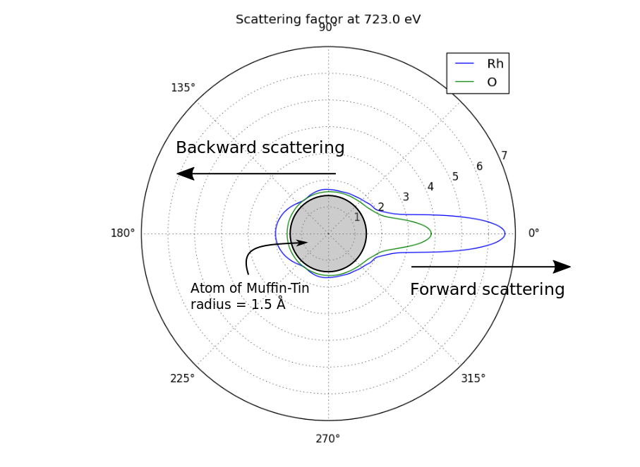
Polar representation of the scattering factor

Let an Oxygen atom being adsorbed at a distance \(z_0\) of an fcc site of the (111) Rh surface. and compute the \(\theta-\phi\) scan for different values of \(z_0\). You can see on the stereographic projection 3 bright circles representing fringes of constructive interference between the direct O(1s) photoelectron wave and that backscattered by the Rhodium atoms. The center of these annular shapes changes from bright to dark due to the variation of the Oxygen atom height above the surface which changes the path difference.

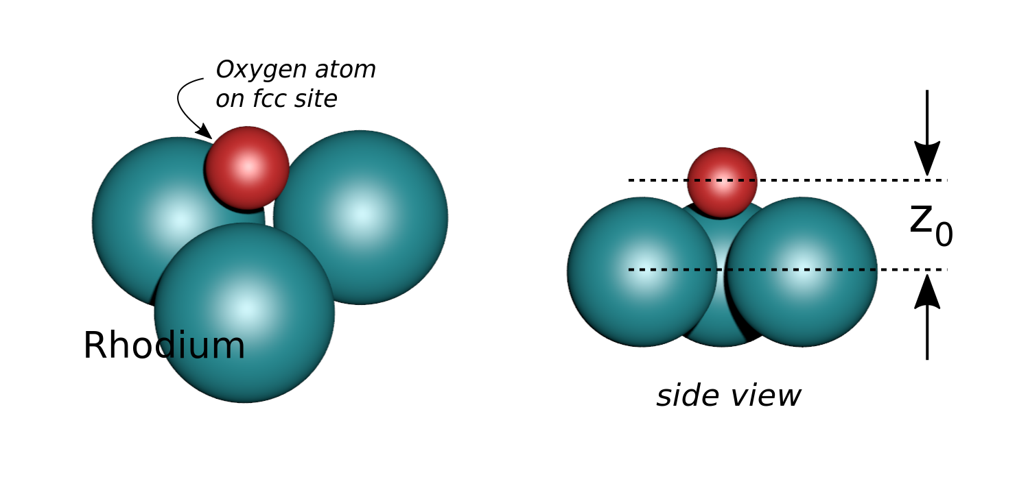
Stereographic projections of O(1s) emission at \(E_k\) = 723 eV for an oxygen atom on top of a fcc site of 3 Rh atoms at various altitudes \(z_0\)

Here is the script for the computation. (download)

# coding: utf8

from msspec.calculator import MSSPEC
from ase.build import fcc111, add_adsorbate
import numpy as np

data = None
all_z = np.arange(1.10, 1.65, 0.05)
for zi, z0 in enumerate(all_z):
    # construct the cluster
    cluster = fcc111('Rh', size = (2,2,1))
    cluster.pop(3)
    add_adsorbate(cluster, 'O', z0, position = 'fcc')
    cluster.absorber = len(cluster) - 1

    # Define a calculator
    calc = MSSPEC(spectroscopy='PED', algorithm='inversion')
    calc.set_atoms(cluster)

    # Compute
    data = calc.get_theta_phi_scan(level='1s', kinetic_energy=723, data=data)
    dset = data[-1]
    dset.title = "{:d}) z = {:.2f} angstroms".format(zi, z0)

data.view()

See also

X-Ray Photoelectron Diffraction in the Backscattering Geometry: A Key to Adsorption Sites and Bond Lengths at Surfaces

T. Gerber, J. Wider, E. Welti & J. Osterwalder, Phys. Rev. Lett. 81 (8) p1654 (1998) [doi]