Photo-Electron Diffraction (PED)
Introduction
In PhotoElectron Diffraction, an incoming photon, with an energy in the X-ray range is absorbed by an atom of the sample. A core electron of the absorbing atom is emitted and will eventually escape from the sample after many scattering events toward a detector. This photo-electron is detected at a given kinetic energy and for a given position (polar angle and azimutal angle) of the detector with respect to the sample (see figure below). The distribution of electrons as a function of the sample polar or azimutal angles contains chemically resolved informations about the crystallography in the immediate proximity of the surface sample. This spectroscopy can also be done on Auger electrons. In this case, the technique is named Auger Electron Diffraction.

The Full picture of a photoelectron diffraction process. a) The geometry of the experiment. b) A view of the multiple scattering process and c) Atomic energy level sketch of the normal and Auger photoemission process.
Quick reference
To quickly start with MsSpec and Python, the easiest way is to read the Learn from tutorials section. Here we summurize all the steps to perform a PED simulation:
Build your cluster (thanks to the ASE python package)
Create a calculator with
MSSPEC()Set the parameters of your calculation.
Attach your cluster to the calculator
Compute a scan
Plot the results
Build your cluster
Building a cluster means creating a list of atoms with their given positions in x, y, z coordinates. It is easily done thanks to the ase Python package.
Because most of spectroscopies have a source and a detector in the same hemispherical space, a cluster
is often shaped as an half sphere. To create such atomic arrangements, special helper functions are provided
in the utils module.
For example to create an MgO cluster:
 1# coding: utf8
 2
 3from ase.build import bulk
 4from msspec.utils import *
 5
 6a = 4.21                                                           # The lattice parameter
 7epsilon = 0.01                                                     # a small usefull value
 8MgO = bulk('MgO', a=a, crystalstructure='rocksalt', cubic=True)    # ASE magic here
 9
10# shaping the cluster in half sphere
11MgO = MgO.repeat((10, 10, 10))
12center_cluster(MgO)
13MgO = cut_plane(MgO, z=epsilon)
14MgO = cut_sphere(MgO, radius=3.*a + epsilon)
15
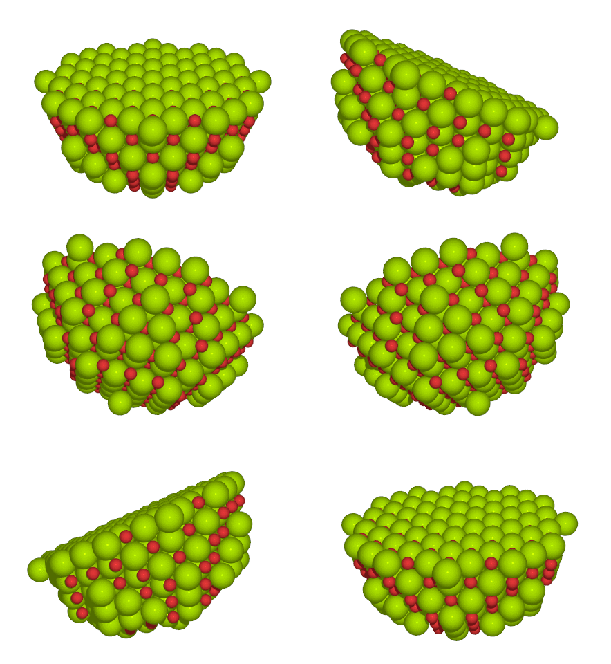
will produce a cluster of 519 atoms like this:

The shape of a typical (yet quite large) cluster used for a calculation (519 atoms of MgO).
Create a calculator
To create a claculator, you will use the calculator.MSSPEC() function. This function takes 4
keyword arguments:
spectroscopy, to specify the kind of spectroscopy. This is a string and can be one of ‘PED’ for PhotoElectron Diffraction, ‘AED’ for Auger Electron Diffraction, ‘APECS’ for Auger PhotoElectron Coincidence Spectroscopy or ‘EXAFS’ for Extended X-Ray Absorption Fine Structure.
algorithm, to choose between the matrix inversion method with the string ‘inversion’ (best suited for lower kinetic energies < 100 eV), or the series expansion technique with ‘expansion’ or the correlation-expansion with ‘correlation’.
polarization to specify the light polarization. ‘linear_qOz’ or ‘linear_xOy’ for a linearly polarized light with the polarization vector in the \((\vec{q}Oz)\) or in the \((xOy)\) plane respectively. Finally choose ‘circular’ for circularly polarized light.
folder. Enter here the name of the folder used for temporary files.
The function returns a calculator object, so for example. To create a calculator for PhotoElectron Diffraction with the matrix inversion method:
calc = MSSPEC(spectroscopy = 'PED', algorithm = 'inversion')
Set the parameters
A calculator has many parameters. They fall into 4 categories:
Muffin-tin parameters, to tweak the potential used for the phase shifts calculation
T-Matrix parameters, to control the T-matrix calculation
Calculation parameters, to tune the multiple scattering calculation: add atomic vibrations, add some filters to speed up the process, control the parameters of the series expansion method…
Spectroscopy dependent parameters. These parameters control – for example – the light source, the detector…
Each set of parameters is accessible through properties of the calculator object. For example, to tweak the interstitial value of the Muffin Tin potential, use:
>>> calc.muffintin_parameters.interstitial_potential = 12.1
To change the source energy, use:
>>> calc.source_parameters.energy = 1253.0
All options are detailed in this section
Attach your cluster
Very easy! Juste use the set_atoms() function like this:
calc.set_atoms(cluster)
Choose the absorber
Set the absorber attribute of your cluster to the index of the atom you want it to be the absorber. For example if the first atom of your cluster is the absorber
cluster.absorber = 0
The best way is to use a function to find the index based on the xyz coordinates of the atom. For example to choose the closest atom of the origin:
cluster.absorber = get_atom_index(cluster, 0, 0, 0)
get_atom_index() is in the utils package so do not forget to import it. The
first argument is the cluster you will look for and the 3 next parameters are the x, y and z
coordinates.
Compute
You can compute 5 kinds of scans in PED spectroscopy:
A polar scan, with the
get_theta_scan()method of the calculator objectAn azimutal scan, with the
MSSPEC.get_phi_scan()methodA stereographic scan, with the
MSSPEC.get_theta_phi_scan()methodAn energy scan, with the
MSSPEC.get_energy_scan()methodThe scattering factor, with the
MSSPEC.get_scattering_factors()method
All these functions are used and detailed in the tutorials.
Plot the results
Normally, the output of the previous functions is a iodata.Data object. You can see
the results by typing:
>>> data = calc.get_theta_scan(...) # a polar scan for example
>>> data.view() # will popup a graphical window